Efficient Training Engine (ETE) for Large Deep Learning Models

Distributed Training

Table of Contents :

There are many ways to efficiently train a large DL model

1. Parallel / Distributed Training

A lot of this content has been derived from this wonderful blog by HuggingFace team on Ultra-Scale Playbook

• Distributed Data Parallelism (DDP)
• Model Parallelism (MP)
  a. Pipeline Parallelism (PP)
  b. Tensor Parallelism (TP)
• Hybrid / Mixed Parallelism
  In real life scenarios we apply all the 3 techniques (DPP to split across data dimension, PP to split across layer dimension, TP to split across hidden dimension) to train a Large Deep Learning Model. This is called 3D Parallelism!!Based on no of GPUs you have you can also combine any two techniques out of these and that is called 2D Parallelism

2. Quantization (Quantization Aware Training — QAT)

In efficient inference engine we learnt how to convert FP32 weights into INT8 weights using quantization after we have trained a model but what if we can directly learn INT8 weights instead of learning FP32 weights during model training itself?? Idea is to perform quantization in one layer and before passing it to second layer perform dequantization such that the second layer does not even know that quantization took place. These are called “fake” quants.

Goal of doing this trick is that this will introduce some quantization error into the MSE loss that is being used to train the regression model. And hence in the process of minimizing MSE loss this quantization error will also get minimized!! Thus we learn good quantized weights during the training process itself!!

3. Low Rank Adaptation (LoRA)

4. Quantised Low Rank Adaptation (QLoRA)

Combining method 2 and 3 i.e. Quantization followed by LORA

Model Parallelism (MP)

Here you split the model across GPUs instead of splitting the data like we saw in Distributed Data Parallelism (DDP). You can divide the model in two ways :

1. Pipeline Parallelism (PP)

Here you cut the model VERTICALLY i.e. layer dimension and distribute it to different GPUs e.g. each GPU is assigned 2 layers of the model (as shown below)

A big issue with this method is GPU utilization. When GPU 4 is performing forward pass on the outputs of GPU3, other GPUs i.e. GPU1, GPU2 and GPU3 are in idle state. Now imagine you are using 1000s of GPU in a big architecture then you can imagine the amount of idle GPUs. This similar GPU idle time issue is observed during backward pass too. Below diagram illustrates this

An example of Pipeline parallelism for a model with 16 layers distributed across 4 GPUs. The numbers correspond to the layer IDs.

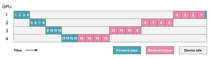
The GPU idle time is indicated in grey and usually called the “bubble”

To tackle this issue i.e. to reduce the bubble size researchers introduced various ideas :

All-Forward-All-Backward (AFAB) Schedule

Here the idea was that we split our batch (dataset) into smaller bit-sized portions which can be processed in parallel, like we did before in data parallel. Now when the second GPU is busy processing micro-batch 1, the first GPU can already start processing micro-batch 2. Here is a schedule using 8 micro-batches:

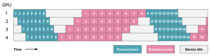
The above schedule is called the all-forward-all-backward (AFAB) schedule as we first do all forward passes and then only all-backward passes.

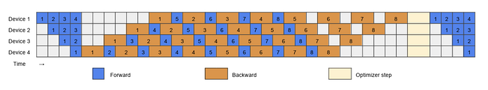
One-Forward-One-Backward (1F1B) Schedule

This schedule is called one-forward-one-backward (1F1B) as the middle/steady state involves alternatively performing one forward and one backward pass. The general idea is to start performing the backward pass as soon as possible. The schedule looks like this:

If you count carefully you’ll see that the bubble still has the same size so our training efficiency is not significantly improved. However we only need to store activations for pp micro-batches (where pp is the degree of pipeline parallelism) instead of mm (where mm was the number of microbatches) which can reduce the activation memory explosion we had in the AFAB schedule. As a consequence we can add more microbatches which then will actually reduce the bubble.

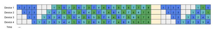
Zero Bubble Schedule

The base observation of ZeroBubble Paper is that the backward pass through a matrix multiplication actually involves two separated operations: backward operation for the inputs (B) and the backward operation for the weights (W).

While the output of B, the backward pass for the input, is necessary for performing the backward pass of the lower layers, the backward pass of the weights, W, is not necessary for the rest of the backward pass and generally only needs to be performed before the optimiser step. You can notice this in the computational graph of a Neural Network.

This means W can be flexibly scheduled anywhere after the corresponding B of the same stage. This allows for strategic placement of W to fill the pipeline bubbles.

Classical 1F1B schedule : interleaving forward and backward pass but keeping a coarse-grained backward pass.

Zero Bubble-H1 Schedule :splitting the backward operation in a “B” and a “W” finer-grained operations.

2. Tensor Parallelism (TP) / Context Parallelism (CP)

Here you cut the model HORIZONTALLY i.e. hidden dimension and distribute it to different GPUs

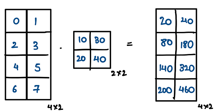
Now we know that each layer is nothing but matrix multiplication and we are dividing the matrix multiplication across 2 GPUs in this case. There are two ways to divide this matrix multiplication across GPUs

Column Tensor Parallelism / Column Linear Parallelism

We’ll copy the complete input matrices to each gpu, using broadcast operation, and split the weight matrix into columns. The inputs are then multiplied with the partial weight matrices, and the results are finally combined using an all-gather operation.

Column Linear Parallelism — note that while combining you just concatenate !!

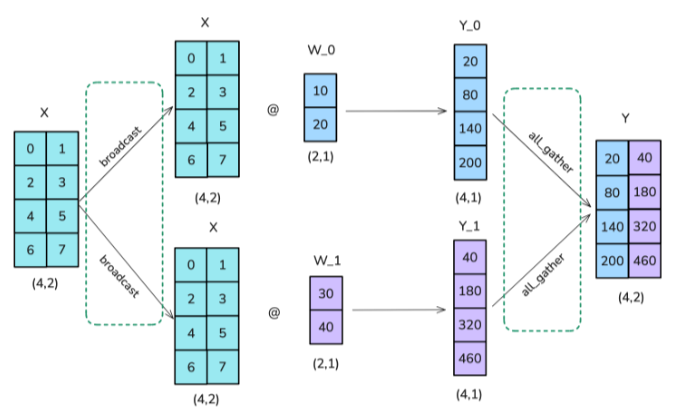
Note : Here we are showing column parallelism across only 2 GPUs, if we have N GPUs then we divide our W into N shards

Tabular-Cross-Sectional-Modelling/modelling/distributed_training/column_tensor_parallel.py at main…

Row Tensor Parallelism / Row Linear Parallelism

In column tensor parallel we split our weight matrix into chunks of columns, here we split the weight matrix into chunks of rows. However, this also requires us to split the inputs, which needs a scatter operation rather than a broadcast as used in column tensor parallel. The results on each gpu are already in the right shape but need to be summed for the final result, thus requiring an all-reduce operation in this scenario.

Row Linear Parallelism — note that while combining you do summation !!

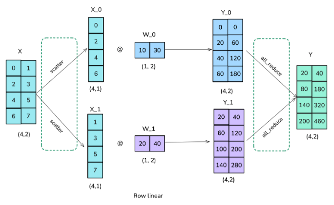
Note : Here we are showing row tensor parallelism across only 2 GPUs, if we have N GPUs then we divide our X and W into N shards

Tabular-Cross-Sectional-Modelling/modelling/distributed_training/row_tensor_parallel.py at main ·…

Combining Column Tensor Parallelism and Row Tensor Parallelism

Now in real life situations where we have large networks to train we do following successive matrix multiplication operation in Neural Network

So now question is how should we combine tensor parallel operations? Like should we apply row tensor parallel to layer1 and then column tensor parallel to layer 2 or vice versa?? In total we have following possibilities

• Row Tensor Parallel + Column Tensor Parallel
• Column Tensor Parallel + Row Tensor Parallel
• Column Tensor Parallel + Column Tensor Parallel
• Row Tensor Parallel + Row Tensor Parallel

To choose which one of the above is most optimal, we use #communication as metric. The method which has the least communication overhead is the best method!!

It turns out that Column Tensor Parallel + Row Tensor Parallel has the least communication overhead (only 2 as shown in below figure) and hence is the best choice !!

Tensor Parallelism using Column Tensor Parallel followed by Row Tensor Parallel

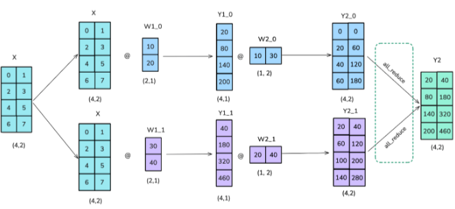
Note : Calculations for Row Tensor Parallel in above image is wrong